Example 1

|
Example 1

|
|
Example 2

|
Example 3
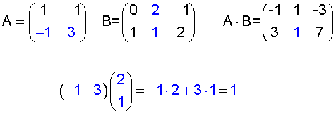
|
exercise 1 problem 1.1
exercise 2 problem 1.2
1.2 Determinants.
The determinant of an squared matrix is a numeric value
computed from the entries of the matrix. It provides information about
the linear dependencies among its rows
or columns.
On the other hand, the unsigned determinant is also the volume
of the solid limited by the rows (alternatively, columns) of the matrix, when we think
of them as a set of vectors with common origin.
Furthermore, the sign of the determinant informs about the particular
orientation induced by a vectorial basis on a
geometrical space.
Determinat computing.
The determinant of an squared nxn matrix is the (signed) sum of all possible products of
n different entries of the matrix, that involve exactly only one entry per row and one entry per column
Example 4 determinant 2x2.

|
Example 5 determinant 3x3 (estrella).

|
Example 6 determinant nxn (desenvolupant
per files o columnes).

|
In a similar way, the determinant of three 3-dimensional vectors computes the volume.
As a consequencia, the determinant of two parallel vectors or three coplanary vectors is null.
More generally, the determinant of n linealment dependent vectors is also null.
exercise 3 problem 1.5
1.3 The rank of a matrix.
We define the rank of a matrix to be its number of
linearly independent rows
(or columns)
Two different approachers can be followed in order to compute
the rank of a given matrix A, which are based on either the notion of
determinant, or the Gauss-Jordan
algorithm.
Precisely, a submatrix of A means a smaller matrix obtained from A by deleting some
of the columns and rows.
Computing the rank
The determinant-based approach consists in finding the biggest squared submatrix
of A such that its determinant is not zero.
|
Example 7
|
is a 2x2 submatrix with null determinant. |
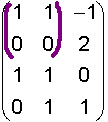
|

|
is a 2x2 submatrix with non null determinant from the same matrix. |
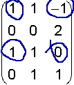
|

|
This is NOT a submatrix, because 1 and 2 do not share the same row. |
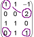
|
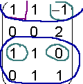
| Example 8 The rank of the matrix in the previous example is 3. Next figure shows a possible sequence of submatrices with non null determinant leading to that fact. |
|
exercise 4 problem 1.6
1.4 Systems of linear equations.
A system of linear equations expresses linear dependencies
among the involved variables ( the so-called unknowns).
Solving the system is the process of finding
the possible values of the unknowns such that satisfy all the equations in the system.
By adding equations to a system we can make it too restrictive
in order to have any solution at all. Conversely, a system with too few equations tend to have
many (infinite) solutions. The reader should take this statement as a rule of thumb rather than
as an exact piece of information. In fact, it is the linear dependencies between equations, rather
than its number, what determines the kind of solutions we can expect.
Some easy examples.
| Problem 9 Find out two numbers such that the first one plus the double of the second equals 6. |
|
Answer. Lets represent the unknown quantities
by two variables, x and y, and lets translate the stated
restriction into mathematical language by writing the equation: x + 2y = 6 .
At a glance, we can find many pairs of values satisfying the required condition, e.g. x=2 and y=2, or x=0 and y=3. Therefore, the solution is not unique. |
| Problem 10 Find out two numbers such that any one of them plus the double of the other equals 6. |
| Answer. In this case, two different constrains are to be imposed leading to a two different equations. As before, we have x + 2y = 6 , but also y + 2x = 6 . The unique solution for that system is x = y = 2 . |
| Problem 11 Find out two numbers such that any one of them plus the double of the other equals 6, and their product equals 8. |
| Answer Three different conditions are to be translated into equations in the present case, which are: x + 2y = 6 , y + 2x = 6 and xy = 8 . Therefore, the number of equations exceedes the number of unknowns. Although this fact in itself does not lead to any particular conclusion, in many cases it goes together with the lack of solutions for the system. That is exactly the case in the present example. There are no values of x and y satisfying all the equations simultaneously. In addition to that, note that the system is NOT linear, as the third equation includes a product of two unknowns. So Gaussian reduction can not be used to solve the system. |
|
| example 12 Going back to the three previous examples, matricial notation looks like: |
|
|
|
|

|

|

|

|

|

|

|
It is not linear. Therefore,
it cannot be expressed as a product of matrices. |
None. |
| exercici 5 problema 1.8 |
Teorema de Rouché-Frobënius
El sistema Ax=b és compatible (o sigui, té solució) si i només si rang(A)=rang(A,b).
A més, la solució depčn de m=n-rang(A) parŕmetres, on n representa el nombre d'incňgnites.
| exercici 6 problema 1.11 |
exemple 13
The ineverse of  is is
 . .
To check that, we only need to compute the product of both matrices:; 
|
exemple 14
The inverse of  does not exist.
This is because the result of multiplying A by any other matrix always has a zero row. does not exist.
This is because the result of multiplying A by any other matrix always has a zero row.

|
example 15 The Gaussian approach.In order to compute the inverse of
 lets write first the 2x4 matrix: lets write first the 2x4 matrix:

We apply now row operations in such a way as to reduce A (the left side) to I, the identity matrix. We will end up with: 
where the right side is exactly the inverse of A, 
|
| exercise 7 problem 1.9 |
example 16 Let us effectively compute the inverse of A in the previous example.
We are looking for a matrix B such that AB=I.


|
| exercise 8 problem 1.10 |